Error Bar
This blog is based on 1 YouTube Vedio by a biologist, explaining how SD and SEM works.
Error bars are everywhere in research papers, how to interprete them? how to calculate them by ourselves?
There are two kind of error bars.
- Sample error of the mean (
SEM) - Standard Deviation (
SD)
An Example
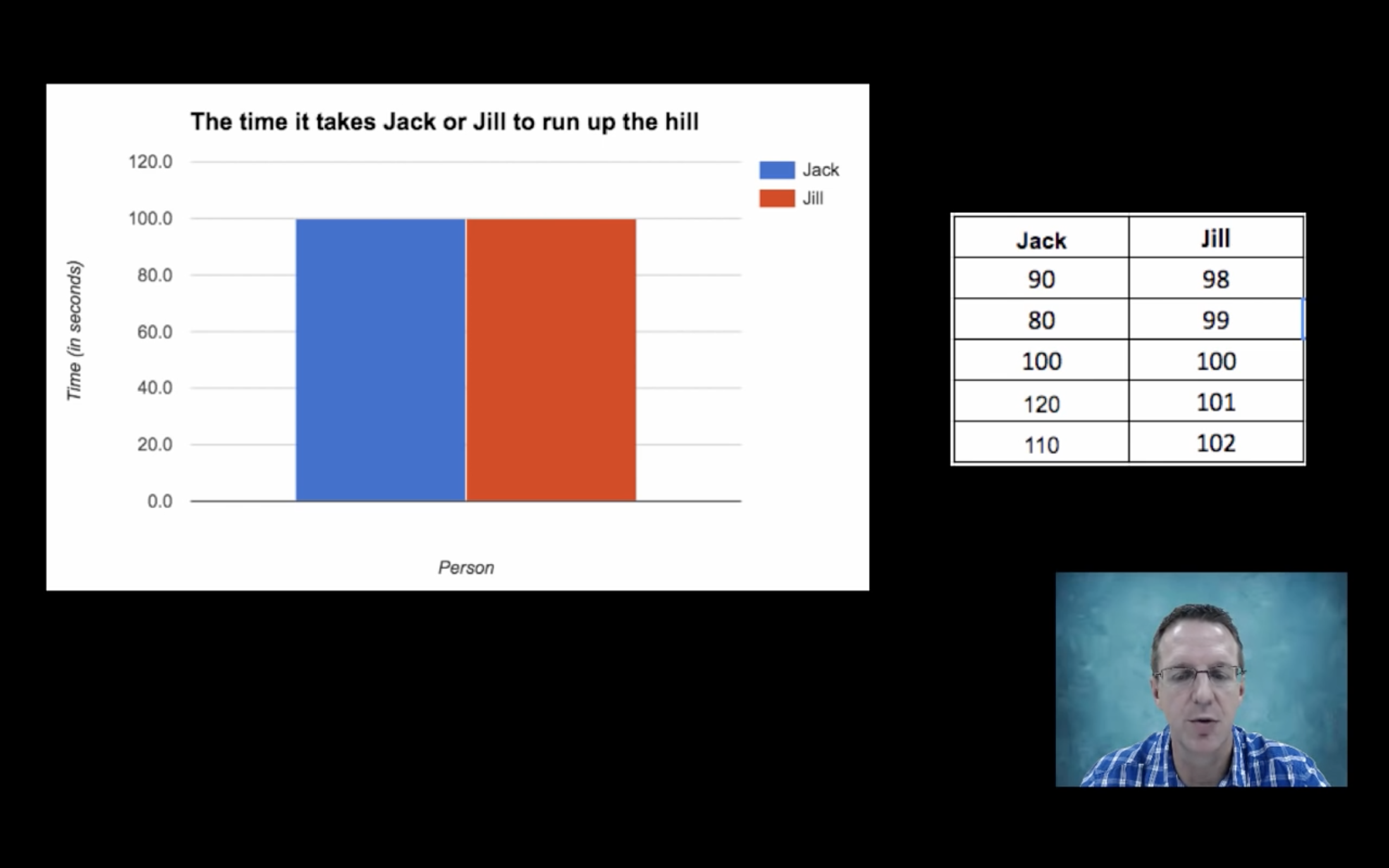
Suppose we want to know who runs up the hill faster, Jack or Jill?
Now we conduct an experiment with 5 trials, for both Jack and Jill.
Evidently, Jack’s speed is more variable, i.e., in this experiment, the SD of Jack’s climbing time is larger.
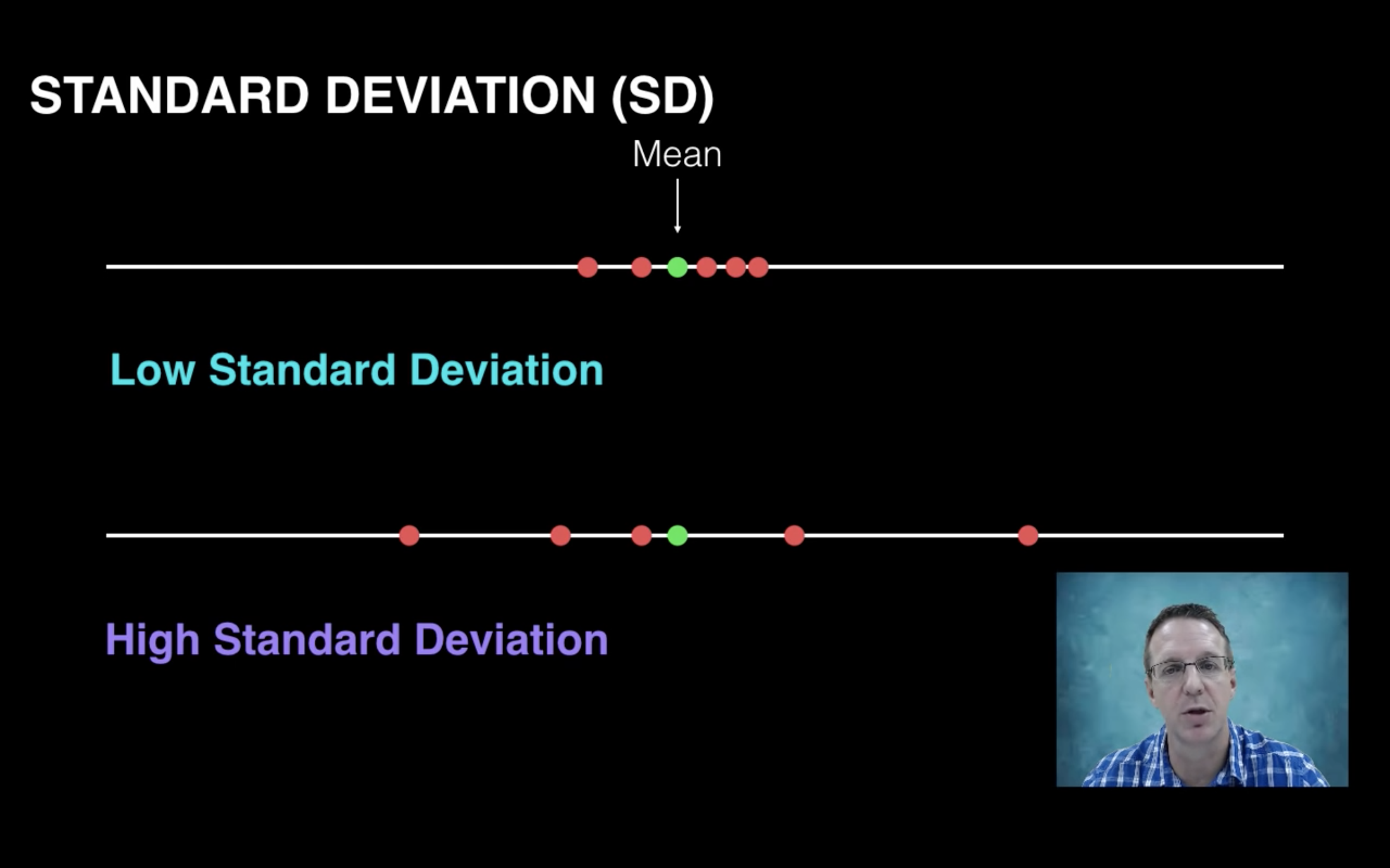
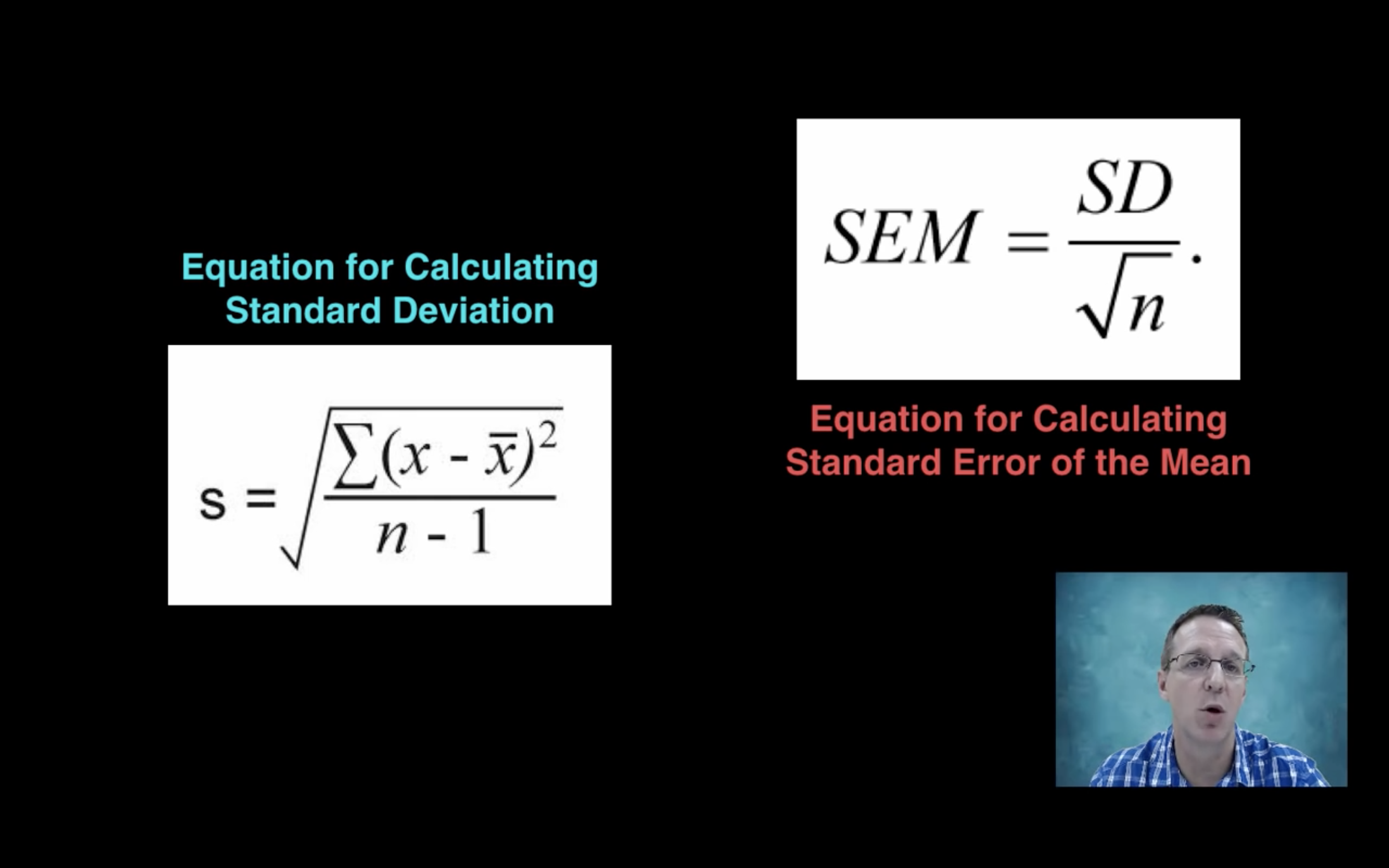
SD
SD is a measure of variability of a set of samples, {s1,s2…}
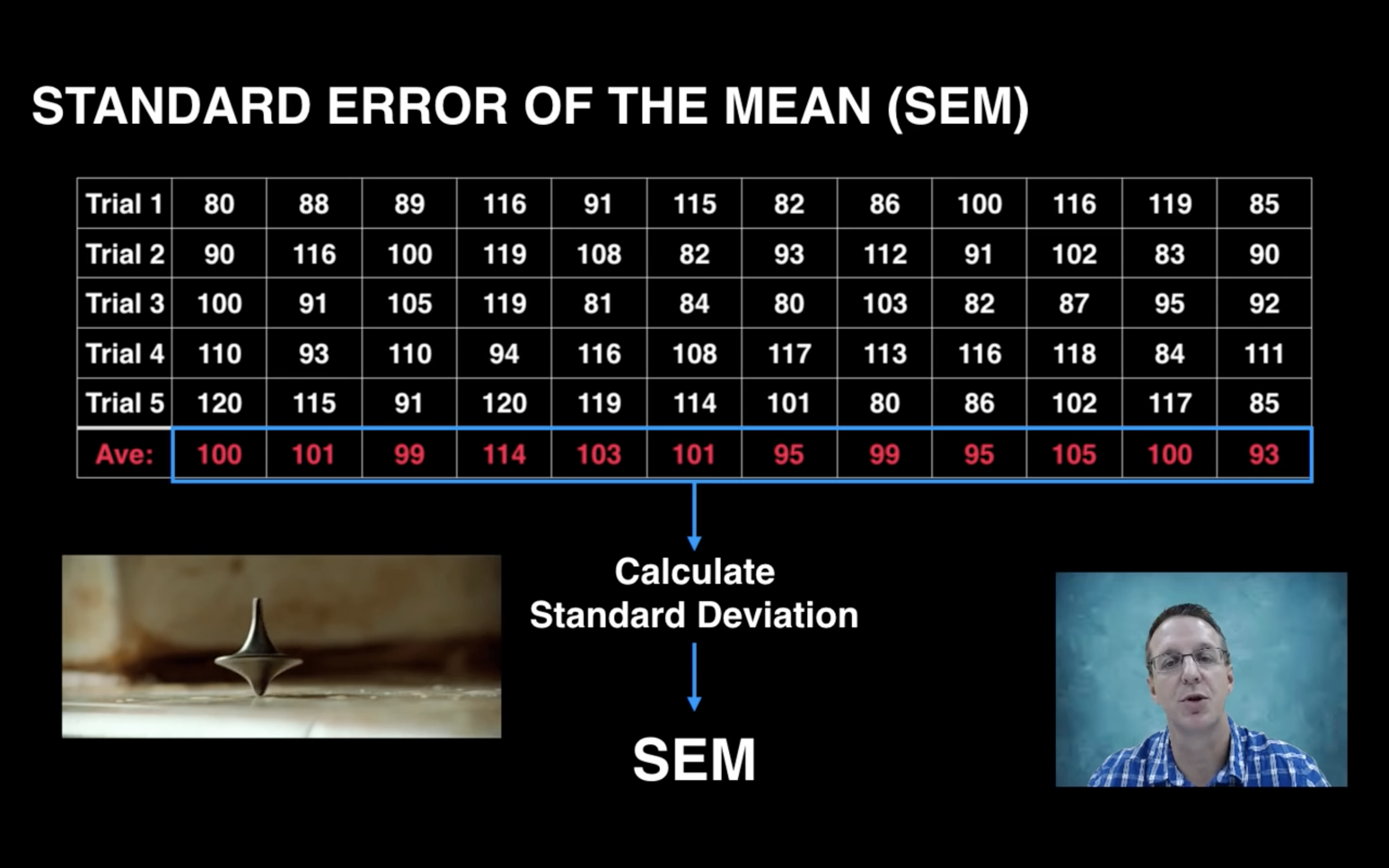
SEM
Then we conduct 12 experiments, each with 5 trials. That’s a lot of data.
By calculating the SD of each sample mean, we have true SEM.
However, this requires too much effort, is there a way to estimate SEM instead?
![]()
![]()
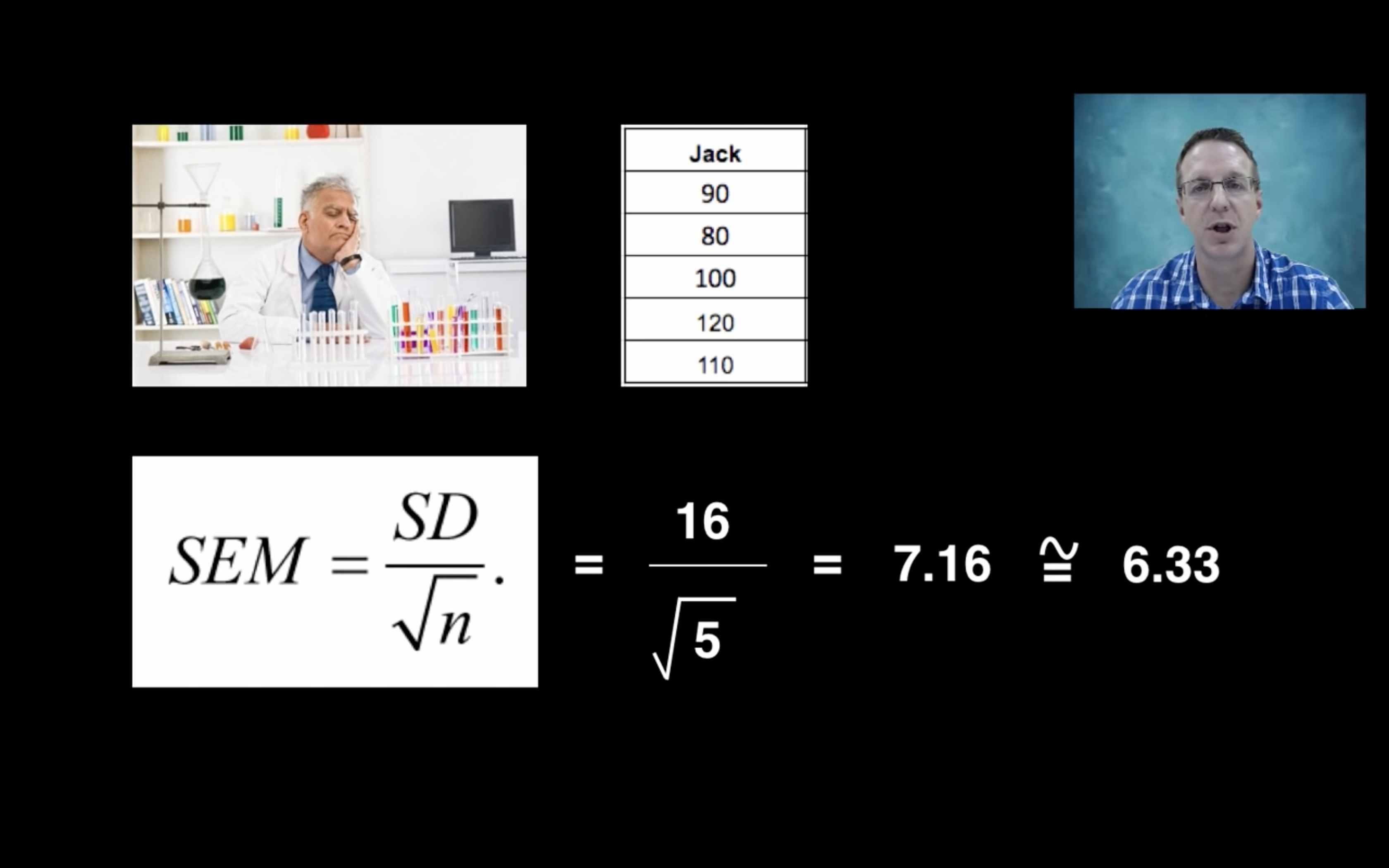
Thankfully, there is one estimator for SEM!
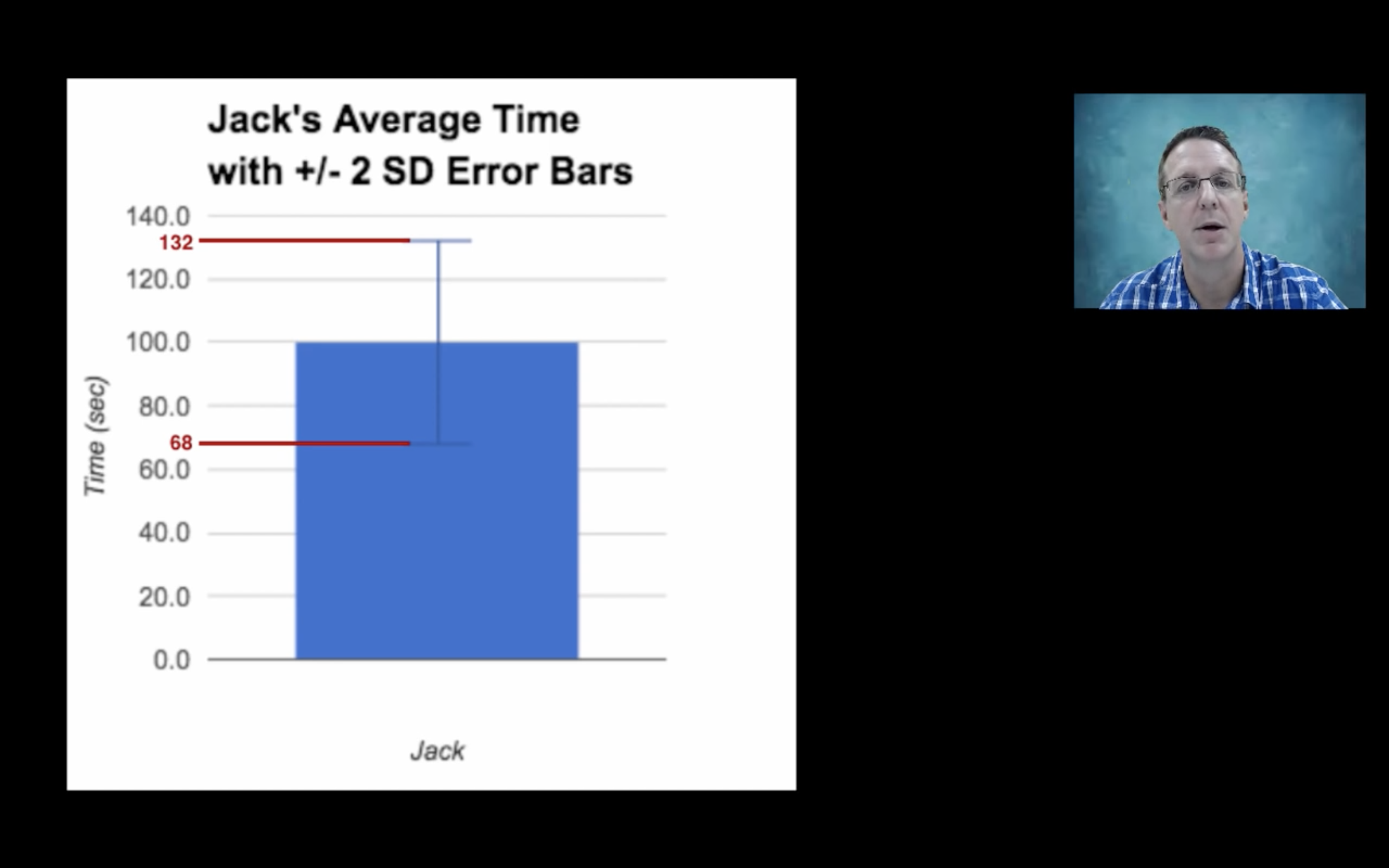
Interprete our result
Now that we have both SD and SEM, we know meaning of two different error bars.
Recall if X ~ N(mu, sigma), P(X in [mu-2sigma, mu+2sigma]) = 95%
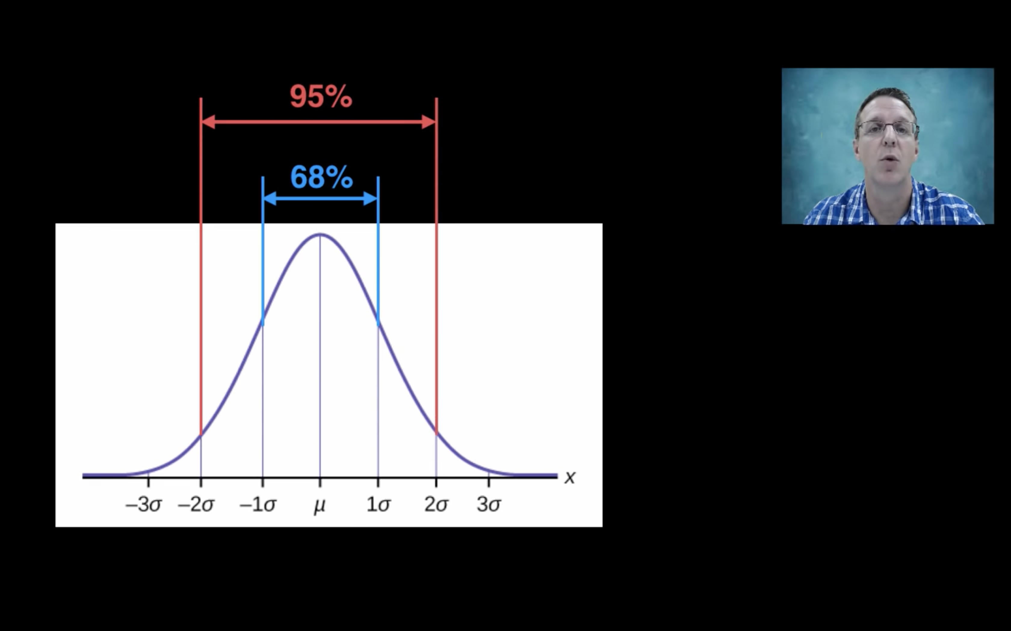
Using SD error bar, we know the variability of our data in this experiment.
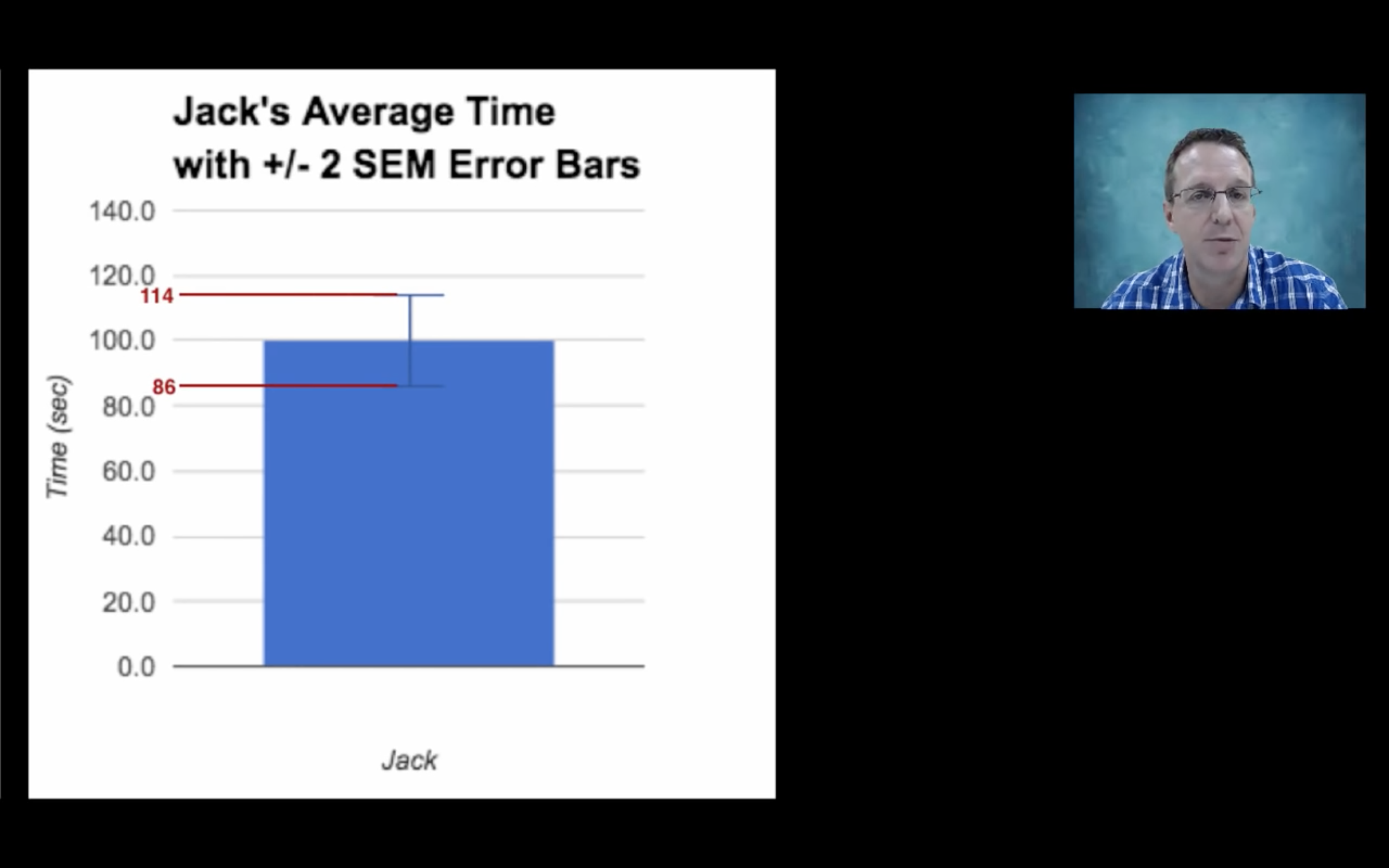
While with SEM error bar, we estimate how far our calculated mean is from our true mean, that’s where the name “sample error of the mean” comes from.
Another instance
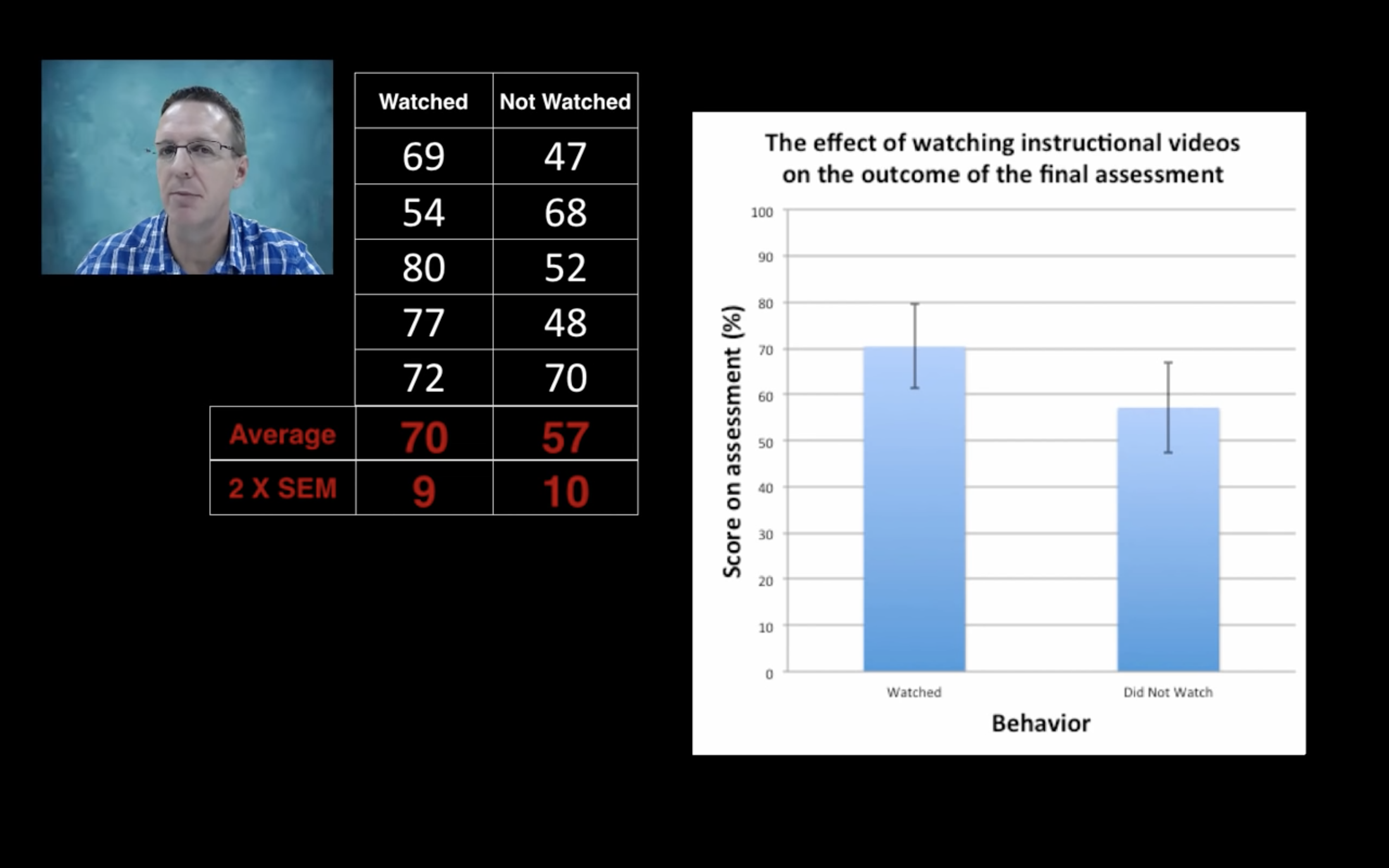
Purpose: study whether watching instruction vedios affects outcome of final exam or not.
Which one is preferred? SD or SEM?
The answer is SEM.Because we do not care about the variability of score within two groups of students.
If we randomly choose 5 students from each group, the two error bars span too much, we don’t have much confidence about the difference between groups.
However, if we collect more samples, the variability doesn’t change much.
Here comes the most amazing part.
Recall the SEM ~= SD/sqrt(number of trials)
Although SD doesn’t change much, SEM decreases!
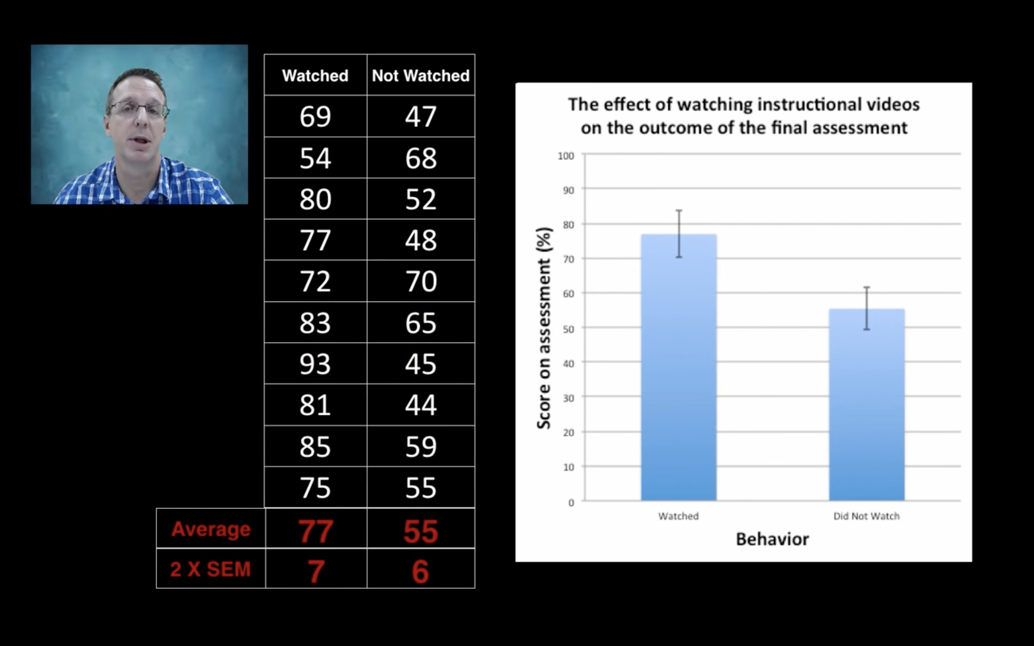
This means we have more confidence on the difference! That’s the context when we talk about Confidential Level

Conclusion
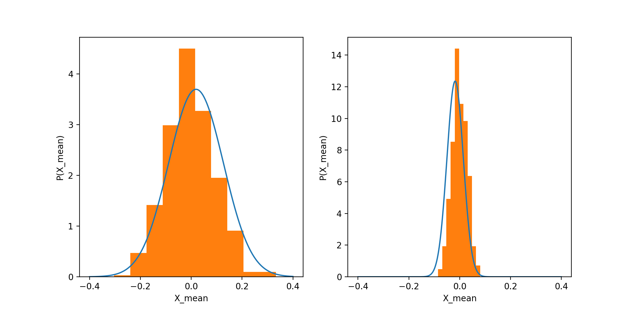
Assume each sample is from a normal distribution with SD. Then the mean of samples in an experiment is also a random variable, its PDF is also a normal distribution, whose SD is what we call SEM.
As the number of our samples grows, SEM decreases, so this normal distribution gets narrower and narrower. Then we have more confidence that the mean we get is close to the true mean.
Python Code
import numpy as np
import matplotlib.pyplot as plt

def SEM_cal(n_sample, n_expt):
    xx =  np.zeros((n_sample, n_expt))
    std = np.zeros(n_expt)
    for i in range(n_expt):
        xx[:,i] = np.random.normal(0, 1, n_sample)
        std[i] = np.std(xx)
    x_means = np.mean(xx, axis=0)
    SEM = np.std(std)
    return (x_means, SEM)

def SEM_estimate(n_sample):
    xx = np.random.normal(0, 1, n_sample)
    return np.mean(xx), np.std(xx)/np.sqrt(n_sample)

def mean_distribution(n_sample, ax):
    n_expt = 500
    mu, sigma = SEM_estimate(n_sample)
    bins = np.linspace(-0.4, 0.4, 1000)
    p_s = [1/(sigma*np.sqrt(2 * np.pi)) * np.exp(-(bin-mu)**2 / (2*sigma**2)) for bin in bins]
    ax.plot(bins, p_s)

    x_means,SEM = SEM_cal(n_sample, n_expt)
    ax.hist(x_means, normed = True)
    ax.set_xlabel("X_mean")
    ax.set_ylabel("P(X_mean)")

fig1 = plt.figure(1)
ax1 = fig1.add_subplot(121)
ax2 = fig1.add_subplot(122)

mean_distribution(100,ax1)
mean_distribution(1000,ax2)
plt.show()
The End